Chapter 5 Prophage Loss Rate Parameter Sweep

The following includes the R scripts that we used to generate our graphs for the data where there we did a parameter sweep on the Prophage Loss Rate to determine which values to use in the remainder of our experiments. There was no induction and no direct benefit for hosts with lysogenic phage.

5.1 Gather Settings and Treatments

General settings

plr_folder <- "Data/PLR_parameter_sweep/" #Folder where datafiles are 
plr_treatments <- c("PLR") #Names of the treatments being tested - should match what is in filenames

Stacked histogram settings

lysis_separate_by <- "PLR" #Facet wrap lysis chance stacked histogram by Prophage Loss Rate

#How lysis chance stacked histogram bins should be collapsed and renamed
lysis_histogram_bins <- c(Hist_0.0 = "0 to 0.2 (Highly lysogenic)",
                          Hist_0.1 = "0 to 0.2 (Highly lysogenic)",
                          Hist_0.2 = "0.2 to 0.4 (Moderately lysogenic)",
                          Hist_0.3 = "0.2 to 0.4 (Moderately lysogenic)",
                          Hist_0.4 = "0.4 to 0.6 (Temperate)",
                          Hist_0.5 = "0.4 to 0.6 (Temperate)",
                          Hist_0.6 = "0.6 to 0.8 (Moderately lytic)",
                          Hist_0.7 = "0.6 to 0.8 (Moderately lytic)",
                          Hist_0.8 = "0.8 to 1.0 (Highly lytic)",
                          Hist_0.9 = "0.8 to 1.0 (Highly lytic)")

5.2 Collect and Munge Data

Gather filenames

plr_all_filenames <- list.files(plr_folder)

plr_freeliving_filenames <- str_subset(plr_all_filenames, "FreeLivingSyms")
plr_hostval_filenames <- str_subset(plr_all_filenames, "HostVals")
plr_lysischance_filenames <- str_subset(plr_all_filenames, "LysisChance")
plr_phagevals_filenames <- str_subset(plr_all_filenames, "SymVals")

Combine time series data for all subsets of datafiles

plr_freeliving <- combine_time_data(plr_freeliving_filenames, plr_folder, plr_treatments)
plr_hostvals <- combine_time_data(plr_hostval_filenames, plr_folder, plr_treatments)
plr_lysischances <- combine_time_data(plr_lysischance_filenames, plr_folder, plr_treatments)
plr_phagevals <- combine_time_data(plr_phagevals_filenames, plr_folder, plr_treatments)

Rearrange time series data into stacked histogram data

plr_lysis_histdata <- combine_histogram_data(plr_lysischances, 
                                         lysis_separate_by, 
                                         lysis_histogram_bins)

Extract information about average genome values at the end of the runs

plr_final_freeliving <- last_update(plr_freeliving)
plr_final_hostvals <- last_update(plr_hostvals)
plr_final_lysischances <- last_update(plr_lysischances)
plr_final_phagevals <- last_update(plr_phagevals)

5.3 Analyze Data

5.3.1 Summary Stats

plr_lysis_summary_stats <- plr_final_lysischances %>%
  group_by(PLR) %>%
  summarise(final_chance_of_lysis = mean(mean_lysischance))

plr_lysis_summary_stats

## # A tibble: 5 x 2
##   PLR   final_chance_of_lysis
##   <fct>                 <dbl>
## 1 0                    0.0488
## 2 0.025                0.392 
## 3 0.05                 0.856 
## 4 0.075                0.847 
## 5 0.1                  0.806

5.3.2 Wilcox tests

Compare PLR of 0 to PLR 5

bonferroni <- 8
plr_PLR0 <- subset(plr_final_lysischances, PLR == "0")
plr_PLR0.05 <- subset(plr_final_lysischances, PLR == "0.05")

wilcox.test(plr_PLR0$mean_lysischance, plr_PLR0.05$mean_lysischance)$p.value * bonferroni

## [1] 3.437693e-17

5.4 Generate Graphs

5.4.1 Host graphs

Host count

hostcount_plot <- ggplot(data=plr_hostvals,
                         aes(x=update, y=count, 
                             group=PLR, colour=PLR)) + 
  ylab("Host Count") + xlab("Updates") + 
  stat_summary(aes(color=PLR, fill=PLR),
               fun.data="mean_cl_boot", geom=c("smooth"), se=TRUE) + 
  theme(panel.background = element_rect(fill='white', colour='black')) +
  theme(panel.grid.major = element_blank(), panel.grid.minor = element_blank()) +
  guides(fill="none") + scale_colour_manual(values=plasma(nlevels(plr_hostvals$PLR)+2)) + 
  scale_fill_manual(values=plasma(nlevels(plr_hostvals$PLR)+2))

hostcount_plot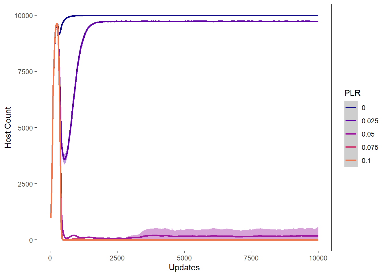

Host cfu count

hostcount_cfu_plot <- ggplot(data=plr_hostvals, aes(x=update, y=cfu_count, 
                                                group=PLR, colour=PLR)) + 
  ylab("Host CFU Count") + xlab("Updates") + 
  stat_summary(aes(color=PLR, fill=PLR),
               fun.data="mean_cl_boot", geom=c("smooth"), se=TRUE) + 
  theme(panel.background = element_rect(fill='white', colour='black')) +
  theme(panel.grid.major = element_blank(), panel.grid.minor = element_blank()) +
  guides(fill="none") + scale_colour_manual(values=plasma(nlevels(plr_hostvals$PLR)+2)) + 
  scale_fill_manual(values=plasma(nlevels(plr_hostvals$PLR)+2))

hostcount_cfu_plot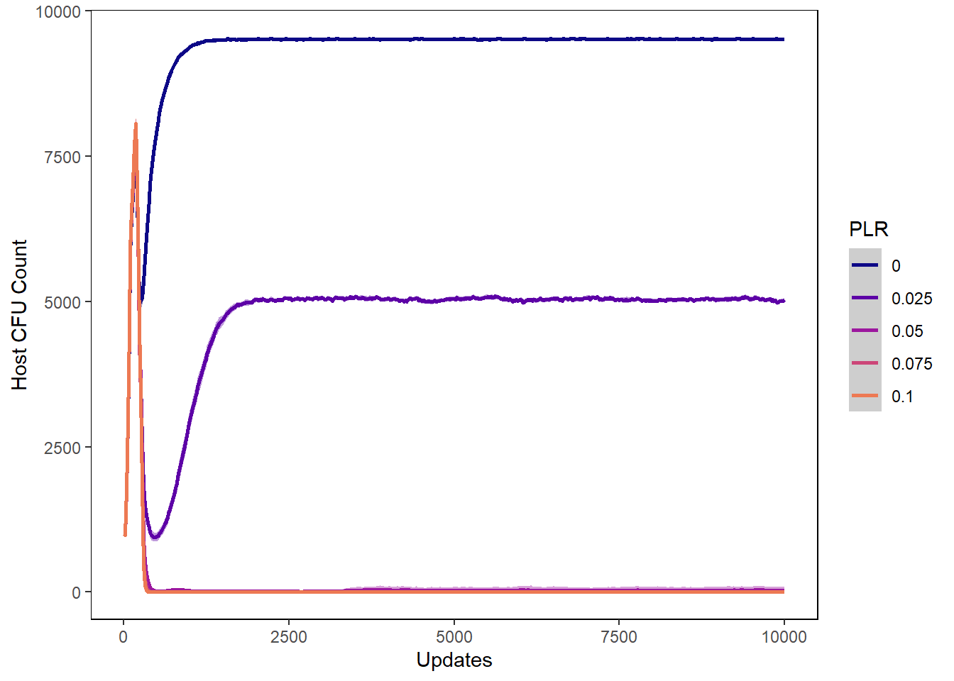

Host uninfected count

host_uninfected_plot <- ggplot(data=plr_hostvals, aes(x=update, y=uninfected_host_count, 
                                                  group=PLR, colour=PLR)) + 
  ylab("Uninfected Host Count") + xlab("Updates") + 
  stat_summary(aes(color=PLR, fill=PLR),
               fun.data="mean_cl_boot", geom=c("smooth"), se=TRUE) + 
  theme(panel.background = element_rect(fill='white', colour='black')) +
  theme(panel.grid.major = element_blank(), panel.grid.minor = element_blank()) +
  guides(fill="none") + scale_colour_manual(values=plasma(nlevels(plr_hostvals$PLR)+2)) + 
  scale_fill_manual(values=plasma(nlevels(plr_hostvals$PLR)+2))

host_uninfected_plot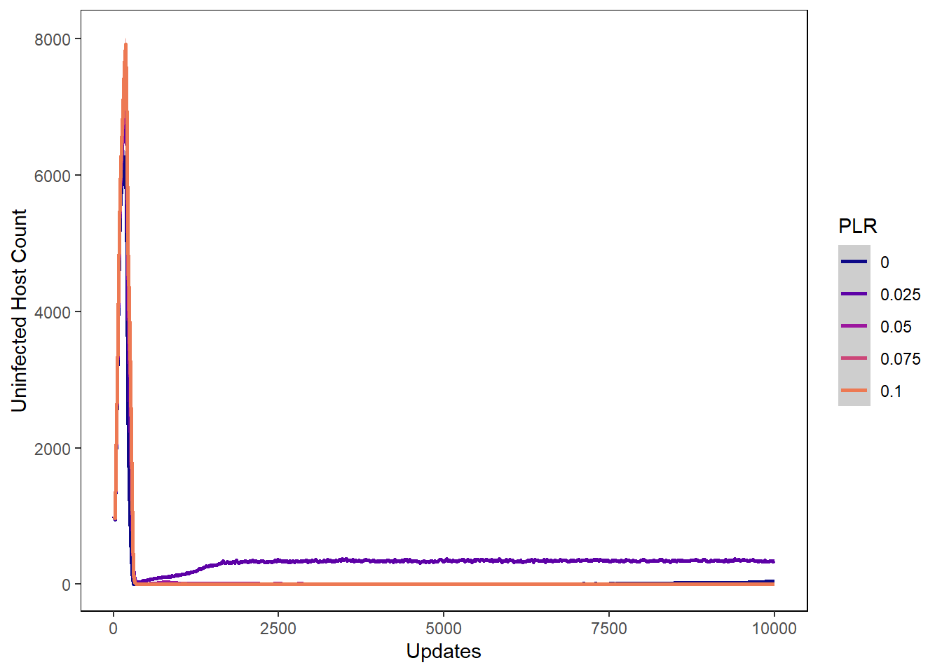

Host int vals

hostvals_plot <- ggplot(data=plr_hostvals, aes(x=update, y=mean_intval, 
                                           group=PLR, colour=PLR)) + 
  ylab("Mean Host Interaction Value") + xlab("Updates") + 
  stat_summary(aes(color=PLR, fill=PLR),
               fun.data="mean_cl_boot", geom=c("smooth"), se=TRUE) + 
  theme(panel.background = element_rect(fill='white', colour='black')) +
  theme(panel.grid.major = element_blank(), panel.grid.minor = element_blank()) +
  guides(fill="none") + scale_colour_manual(values=plasma(nlevels(plr_hostvals$PLR)+2)) + 
  scale_fill_manual(values=plasma(nlevels(plr_hostvals$PLR)+2))

hostvals_plot

## Warning: Removed 31562 rows containing non-finite values (stat_summary).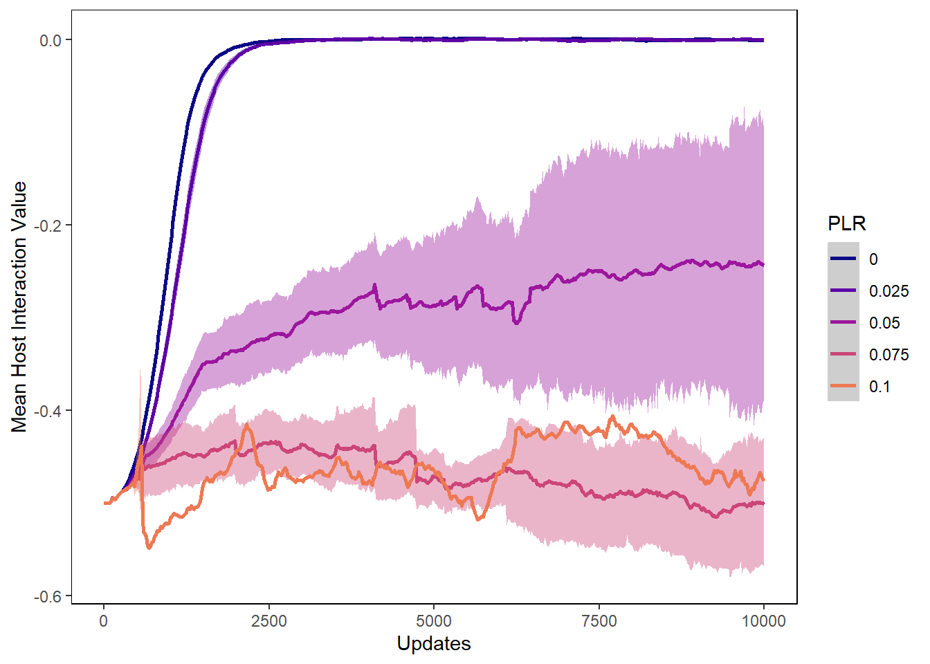

5.4.2 Phage graphs

Phage count

phagecount_plot <- ggplot(data=plr_lysischances,
                          aes(x=update, y=count,
                              group=PLR, color=PLR)) +
  ylab("Phage count") + xlab("Updates") + 
  stat_summary(aes(color=PLR, fill=PLR),
               fun.data="mean_cl_boot", geom=c("smooth"), se=TRUE) + 
  theme(panel.background = element_rect(fill='white', colour='black')) +
  theme(panel.grid.major = element_blank(), panel.grid.minor = element_blank()) +
  guides(fill="none") + scale_colour_manual(values=plasma(nlevels(plr_lysischances$PLR)+2)) + 
  scale_fill_manual(values=plasma(nlevels(plr_lysischances$PLR)+2))

phagecount_plot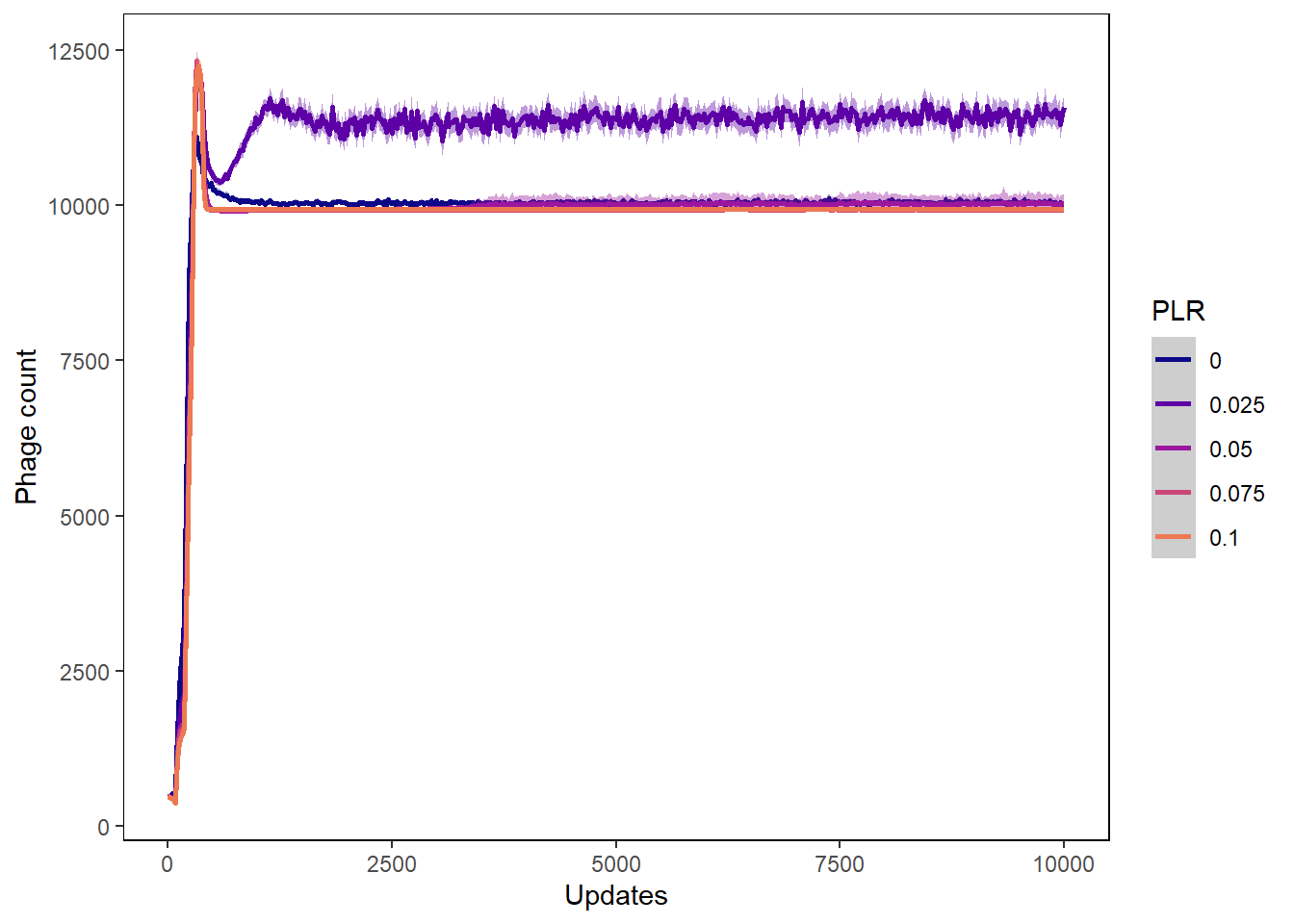

Phage int val

phageintval_plot <- ggplot(data=plr_phagevals, aes(x=update, y=mean_intval,
                                               group=PLR, color=PLR)) +
  ylab("Phage Interaction value") + xlab("Updates") + 
  stat_summary(aes(color=PLR, fill=PLR),
               fun.data="mean_cl_boot", geom=c("smooth"), se=TRUE) + 
  theme(panel.background = element_rect(fill='white', colour='black')) +
  theme(panel.grid.major = element_blank(), panel.grid.minor = element_blank()) +
  guides(fill="none") + scale_colour_manual(values=plasma(nlevels(plr_phagevals$PLR)+2)) + 
  scale_fill_manual(values=plasma(nlevels(plr_phagevals$PLR)+2))

phageintval_plot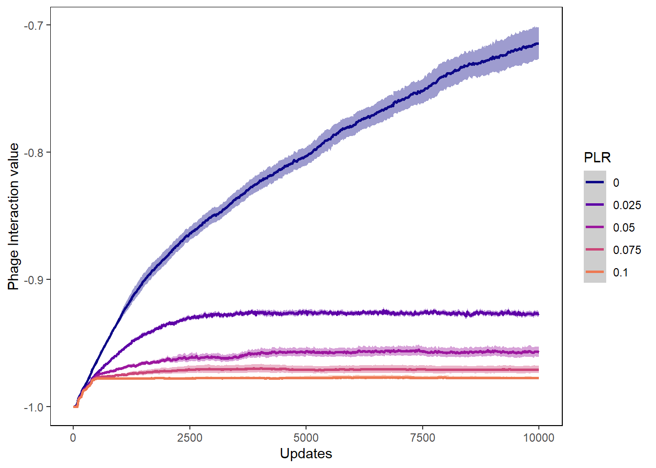

Chance of lysis

lysischances_plot <- ggplot(data=plr_lysischances,
                            aes(x=update, y=mean_lysischance,
                                group=PLR, color=PLR)) +
  ylab("Mean Chance of Lysis") + xlab("Evolutionary Time (Updates)") + 
  stat_summary(aes(color=PLR, fill=PLR),
               fun.data="mean_cl_boot", geom=c("smooth"), se=TRUE) + 
  theme(panel.background = element_rect(fill='white', colour='black')) +
  theme(panel.grid.major = element_blank(), panel.grid.minor = element_blank()) +
  guides(fill="none") + 
  scale_colour_manual(values=plasma(nlevels(plr_lysischances$PLR)+2)) + 
  scale_fill_manual(values=plasma(nlevels(plr_lysischances$PLR)+2))

lysischances_plot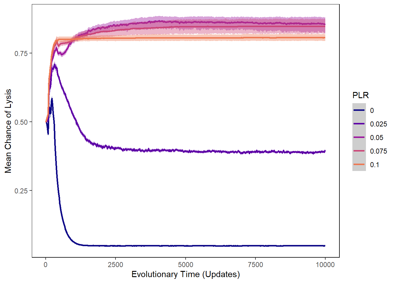

Chance of lysis boxplot

plr_final_lysischances2 <- plr_final_lysischances %>%
  filter(PLR %in% c("0", "0.025", "0.05"))

lysis_boxplot <- ggplot(data = plr_final_lysischances2, 
                              aes(x = PLR, y = mean_lysischance,
                                  group=PLR, color=PLR)) + 
  geom_boxplot(
    width = .25, 
    outlier.shape = NA
  ) +
  geom_point(
    size = 1.3,
    alpha = .3,
    position = position_jitter(
      seed = 1, width = .1
    )
  ) + 
  coord_cartesian(xlim = c(1.2, NA), clip = "off") +
  ylab("Mean Chance of Lysis") + xlab("Prophage Loss Rate") +
  theme(panel.background = element_rect(fill='white', colour='black')) +
  theme(panel.grid.major = element_blank(), panel.grid.minor = element_blank()) +
  guides(fill="none") +
  scale_colour_manual(values=plasma(5)) + 
  scale_fill_manual(values=plasma(5)) +
  scale_y_continuous(labels = scales::percent) +
  theme(legend.position = "none")

lysis_boxplot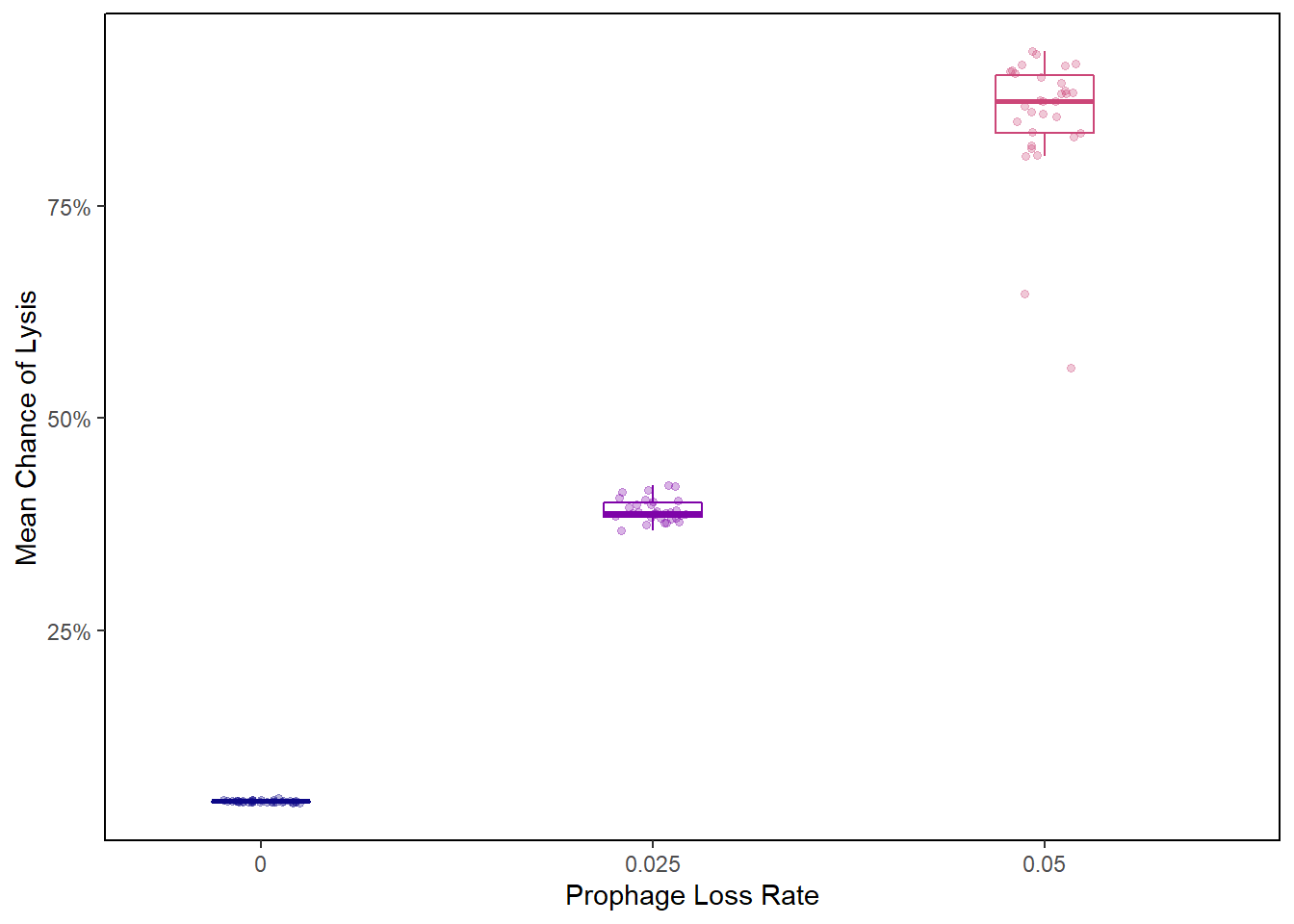

5.4.3 Stacked Histograms

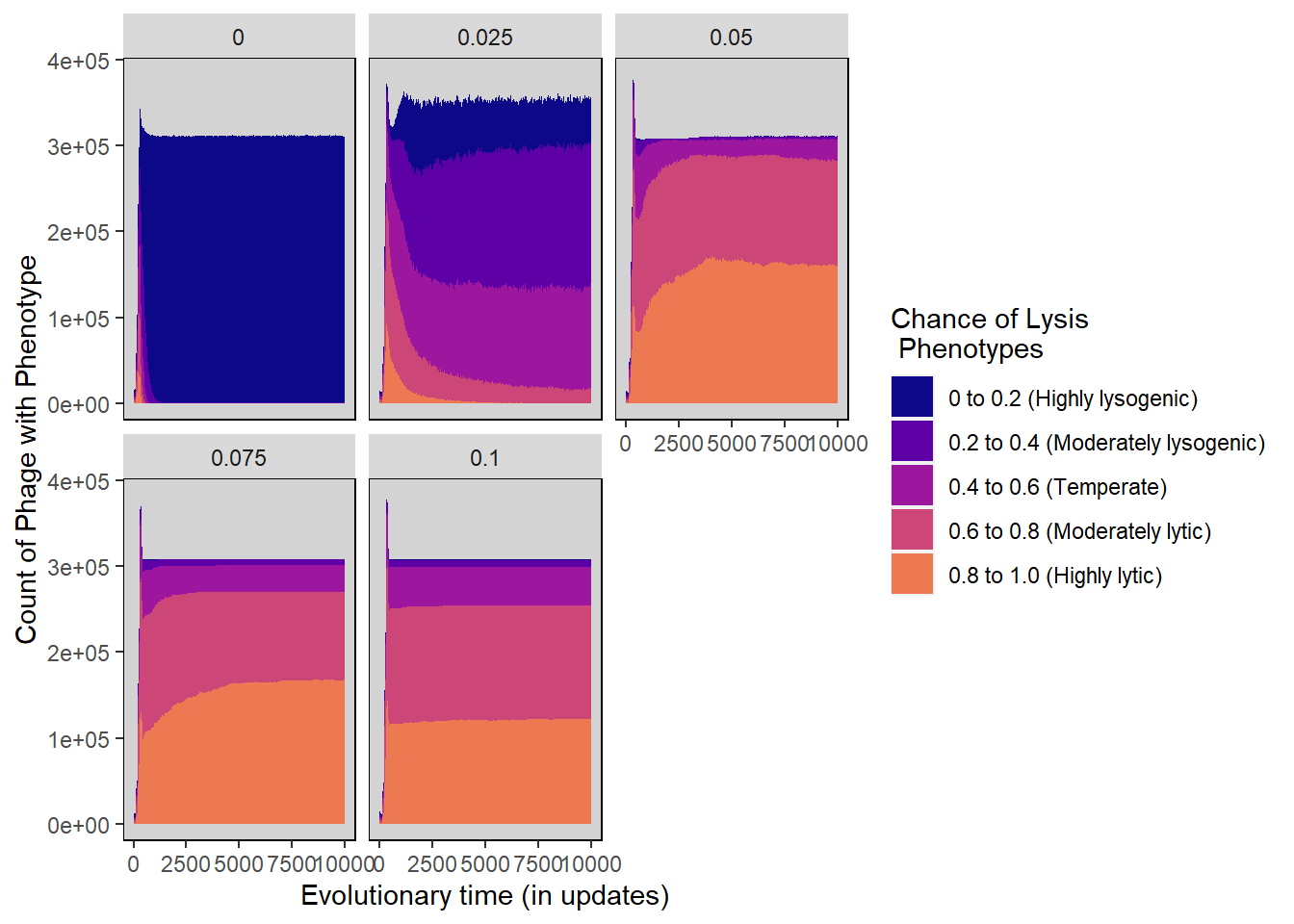
Chance of lysis stacked histogram

lysischance_stackedhistogram <- ggplot(plr_lysis_histdata, 
                                       aes(update, count)) + 
  geom_area(aes(fill=Histogram_bins), position='stack') +
  ylab("Count of Phage with Phenotype") + xlab("Evolutionary time (in updates)") +
  scale_fill_manual("Chance of Lysis\n Phenotypes",values=plasma(nlevels(plr_lysis_histdata$Histogram_bins)+2)) +
  facet_wrap(~treatment) + 
  theme(panel.background = element_rect(fill='light grey', colour='black')) + 
  theme(panel.grid.major = element_blank(), panel.grid.minor = element_blank()) + 
  guides(fill="none") + guides(fill = guide_legend())

lysischance_stackedhistogram